Recurring Neural Networks for Time Series Forecasting

Single-Variate Time Series

Imagine we are loading a csv file with two columns. The first one is a date-time string (called DATE, and the second one is the value we want to forecast. The following command loads the csv file into a dataframe and assigns the date-time info to the index. Setting parse_dates=True ensures the date-time information is read in as a date-time object and not as a string:

df = pd.read_csv('data.csv',parse_dates=True,index_col='DATE')

Assume each row represents a month and that we want as our test sample the last 24 months of data:

test_size = 24
test_ind = len(df) - test_size
train = df.iloc[:test_ind]
test = df.iloc[test_ind:]

Now scale the data:

from sklearn.preprocessing import MinMaxScaler
scaler = MinMaxScaler()
scaled_train = scaler.fit_transform(train)
scaled_test = scaler.transform(test)

and create a time series generator with length of 20 months and a batch size of 1:

from tensorflow.keras.preprocessing.sequence import TimeseriesGenerator
length = 20
batch_size = 1
generator = TimeseriesGenerator(scaled_train,scaled_train,
                           length=length,batch_size=batch_size)

Create the model. Here we will use a Long Short-Term Memory (LSTM) layer. Alternatively we could have used a SimpleRNN layer, but LSTM tends to work better:

from tensorflow.keras.models import Sequential
from tensorflow.keras.layers import LSTM, Dense

n_features = 1

model = Sequential()
model.add(LSTM(100,activation='relu',input_shape=(length,n_features)))
model.add(Dense(1))
model.compile(loss='mse',optimizer='adam')

Let’s now create a validation generator with the test data:

test_generator = TimeseriesGenerator(scaled_test,scaled_test,
                                    length=length,batch_size=batch_size)

Create and early stop callback and train the model:

from tensorflow.keras.callbacks import EarlyStopping
early_stop = EarlyStopping(monitor='val_loss',patience=3)
model.fit(generator,epochs=50,validation_data=test_generator,callbacks=[early_stop])

Plot the history of the loss that occured during training:

loss = pd.DataFrame(model.history.history)
loss.plot()

Finally, to evaluate the model, we can forecast predictions for test data range (the last 24 months of the entire dataset). We have to inverse the scaling transformations:

predictions = []

first_batch = scaled_train[-length:]
current_batch = first_batch.reshape(batch_size,length,n_features)

for i in range(len(test)):
    current_pred = model.predict(current_batch)[0]
    
    predictions.append(current_pred)
    
    current_batch = np.append(current_batch[:,1:,:],[[current_pred]],axis=1)

preds = scaler.inverse_transform(predictions)
test['predictions'] = preds

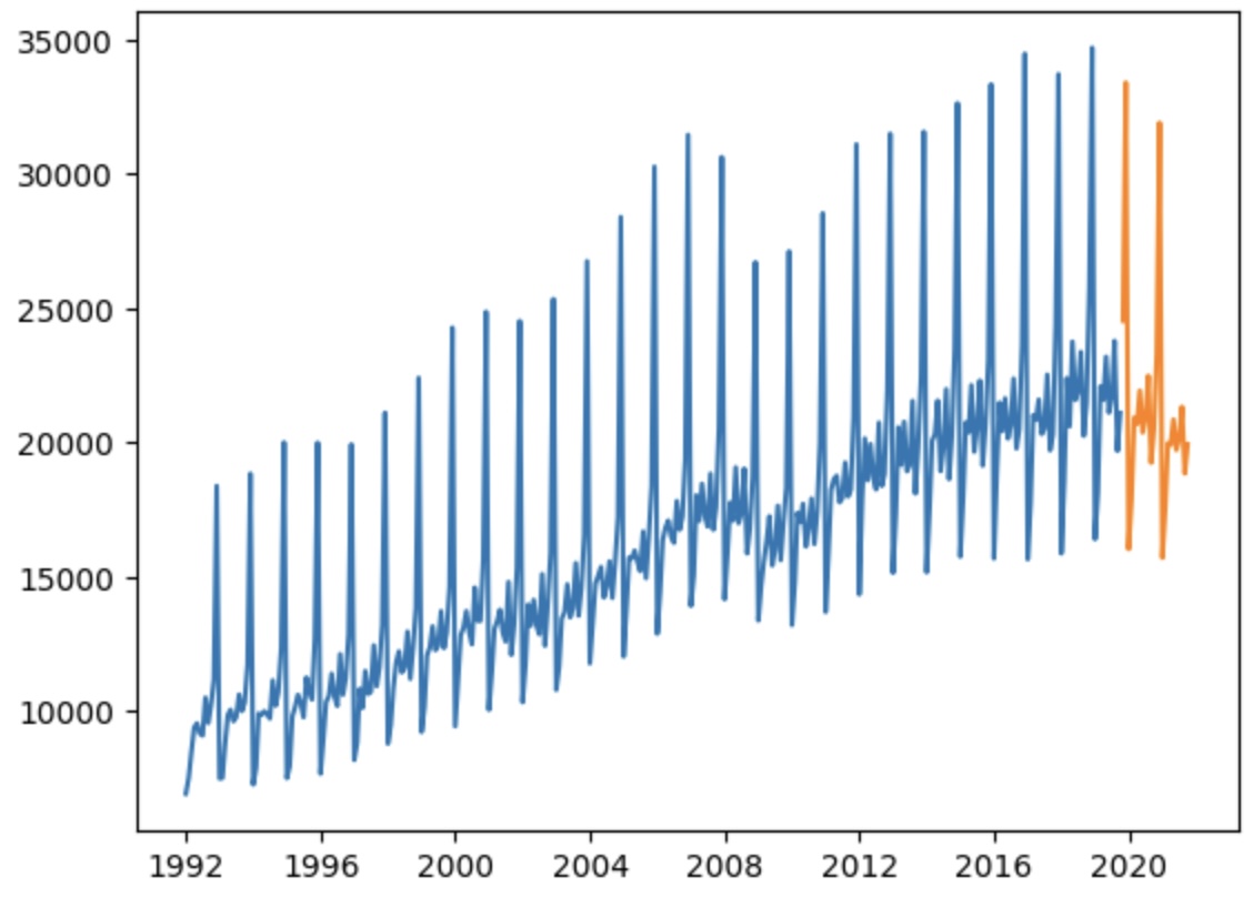
See below an example of forecast (orange) after training on the (blue) data:

Multi-Variate Time Series

The two changes we need here are:

1. Change input shape in LSTM layer to reflect the higher dimensionality
2. Final dense layer should have a neuron per feature.